简单神经网络之验证码识别

  此前虽也做过不少验证码识别的项目（比如微班安全教育和 iSmart 以及智学网的登录），但这些东西图形都比较简单，只用简单的模板匹配就能达到很高的识别率，所以一直也就这么用着，直到有一天碰到了硬点子……

  这网站的验证码长这样：

  随机的颜色、随机的位置、随机的扭曲度、随机的字号……让传统匹配算法有些力不从心，之前虽然有过用 Tesseract 成功识别的案例，不过一是识别率不够高，二是移植脚本时还要额外安装 Tesseract（不同平台的安装方法还不同），感觉怪麻烦的，思来想去……感觉核心技术还是要掌握在自己手中，如果能打造一款针对这个网站设计的验证码识别脚本，应该可大大提升识别的效率和准确度。

---

准备工作

  说干就干，首先设计好框架，神经网络应该只具备单个字符识别的功能，这样会更有利于训练，所以需要先用一些简单的预处理算法将 4 字符的验证码切分为 4 张等大的图片，再分别交给网络进行识别，最后将结果整合起来，作为识别的结果。

将验证码切分为字符

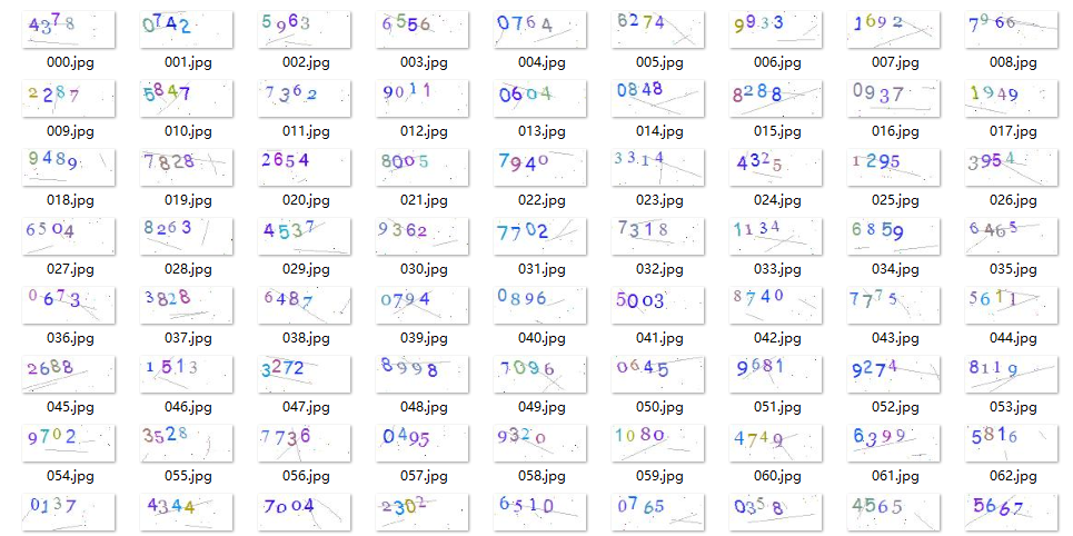
  那么先从最简单的切分部分开始，下载 1000 张验证码图片作为模板和测试用例：

import asyncio
from random import randint
from time import time

import httpx
from loguru import logger


def get_uuid():
    return f'{time()*1000:.0f}{randint(100, 999)}'


async def download_image(count):
    client = httpx.AsyncClient()
    limit = asyncio.Semaphore(4)

    async def internal():
        async with limit:
            try:
                token = (
                    await client.get('https://fangkong.hnu.edu.cn/api/v1/account/getimgvcode')
                ).json()['data']['Token']
                image = await client.get(f'https://fangkong.hnu.edu.cn/imagevcode?token={token}')
            except Exception as err:
                logger.error(repr(err))
                return

        path = f'../data/raw_image/{get_uuid()}.jpg'
        logger.info(f'File saved to: {path}')
        with open(path, 'wb') as fp:
            fp.write(image.content)

    await asyncio.gather(*[internal() for _ in range(count)])
    await client.aclose()


async def main():
    await download_image(1000)


if __name__ == '__main__':
    loop = asyncio.new_event_loop()
    try:
        loop.run_until_complete(main())
    finally:
        loop.close()

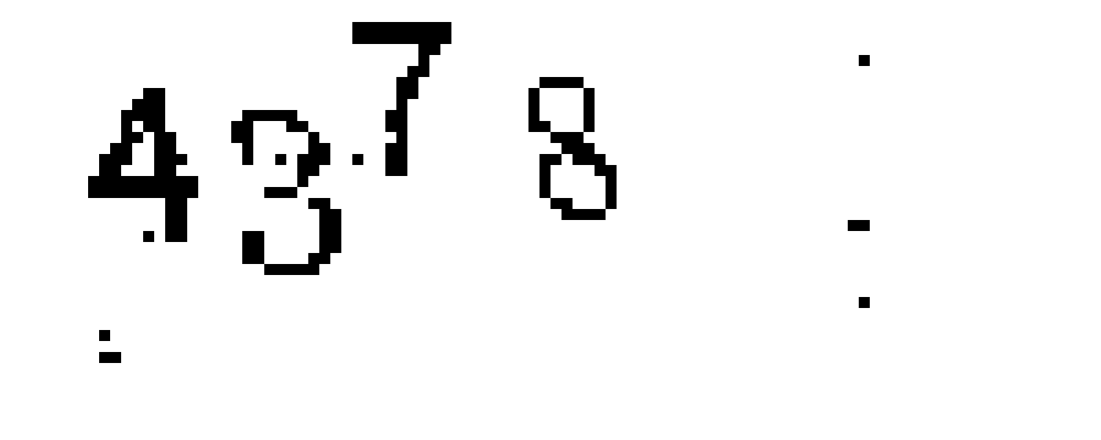
  从模板的内容来看，大部分的文字都位于验证码图片的左上角，自然而然的会想到先对验证码进行裁剪预处理，但究竟需要裁多大一块区域呢？我用一个脚本对所有图片进行了灰度化和叠加处理：

import os
import cv2
import numpy as np
import matplotlib.pyplot as plt

overlay = None

files = os.listdir('../data/raw_image')
for file in files:
    image = cv2.imread(f'../data/raw_image/{file}')
    image = cv2.cvtColor(image, cv2.COLOR_RGB2GRAY)
    if overlay is None:
        overlay = np.zeros(image.shape)
    overlay += image

if overlay is not None:
    overlay = overlay * 255 / np.max(overlay)
    plt.imshow(overlay)
    plt.show()

  最终结果显示：99% 的数字都出现在左上角 67*27 的区域中，所以我们提前裁剪这块区域，以减少后期的计算量

  难点来了！如何让程序将不同的字符区分出来，成为一个值得研究的问题。传统的方法是统计每一竖排上黑色像素的数量（想象一张柱状图），然后采用一根扫描线自下而上不断扫描，直到扫描线上方的「柱状图」连通块数量第一次为 4（即字符数量），但在字符随机倾斜的情况下，继续沿用这样的方法非常容易产生切割错误的问题，我们需要一种更有效的算法来进行字符切分

---

  观察二值化后的验证码，发现每个字符的各个像素之间的关联性并不强，甚至有些字符简直可以用「支离破碎」来形容，这意味着如果直接进行搜索，将很容易出现错误。所以考虑首先使用 3×5 的算子对图片进行高斯模糊处理，然后再进行一次二值化，从而将每个字符「粘连」起来，处理之后的图片长这样：

  差不多就要开始切分了，首先对上一步得到的图像进行深度优先搜索，找出所有连通量在 20～150 的黑色像素连通块并进行标记，最后进行一次判断，如果找到符合条件的像素块（即字符）数量为 4，则按照记录进行切分，将每个字符缩放到 10×15px 的区域并置中，最后做一次 3×3px 的高斯模糊：

import os

import cv2
import matplotlib.pyplot as plt
import numpy as np

DIGITS = 4  # 验证码的字符数
WIDTH, HEIGHT = 67, 27  # 从左上角裁剪的长宽
BINARY_THRESHOLD = 180  # 二值化的阈值
BLUR_CORE_SIZE = (3, 5)  # 高斯模糊核心大小
BLUR_BINARY_THRESHOLD = 210  # 高斯模糊后再次二值化的阈值
MIN_BLOCK_SIZE, MAX_BLOCK_SIZE = 20, 150  # 像素块大小范围
DIGIT_WIDTH, DIGIT_HEIGHT = 10, 15  # 验证码数字尺寸


def mark(image, mask):
    shape = image.shape
    flag = np.zeros(image.shape, dtype=np.uint8)

    def dfs(x, y, depth, flow):
        # noinspection PyChainedComparisons
        if 0 <= x < shape[0] and 0 <= y < shape[1] and mask[x, y] == 0 and not flag[x, y]:
            flow.append((x, y))
            flag[x, y] = 1
            count = 1
            for way in ((-1, 0), (0, 1), (0, -1), (1, 0)):
                count += dfs(x + way[0], y + way[1], depth + 1, flow)
            return count
        else:
            return 0

    results = []
    for i in range(image.shape[0]):
        for j in range(image.shape[1]):
            if flag[i, j]:
                continue
            if mask[i, j] == 0:
                pixels = []
                if MIN_BLOCK_SIZE <= dfs(i, j, 0, pixels) <= MAX_BLOCK_SIZE:
                    results.append((
                        image[
                            min(x[0] for x in pixels):max(x[0] for x in pixels),
                            min(x[1] for x in pixels):max(x[1] for x in pixels)
                        ],
                        sum(x[1] for x in pixels) / len(pixels)
                    ))
            flag[i, j] = 1

    if len(results) != 4:
        return None

    results.sort(key=lambda x: x[1])
    return [x[0] for x in results]


def split(image):
    image = cv2.cvtColor(image[:HEIGHT, :WIDTH], cv2.COLOR_RGB2GRAY)
    binary = cv2.threshold(image, BINARY_THRESHOLD, 255, cv2.THRESH_BINARY)[1]
    mask = cv2.threshold(
        cv2.GaussianBlur(binary, BLUR_CORE_SIZE, 0),
        BLUR_BINARY_THRESHOLD, 255, cv2.THRESH_BINARY
    )[1]

    digits = mark(image, mask)

    if digits is None:
        return None

    for i, digit in enumerate(digits):
        scale = max(digit.shape[0] / DIGIT_HEIGHT, digit.shape[1] / DIGIT_WIDTH)
        digit = cv2.resize(
            digit, (int(digit.shape[1] / scale), int(digit.shape[0] / scale)),
            interpolation=cv2.INTER_LANCZOS4
        )
        height, width = digit.shape
        background = np.full((DIGIT_HEIGHT, DIGIT_WIDTH), 255)
        left, top = (DIGIT_WIDTH - width) // 2, (DIGIT_HEIGHT - height) // 2
        background[top:top+height, left:left+width] = digit

        digits[i] = background

    return digits


def main():
    path = '../data/raw_image'
    for file in os.listdir(path):
        image = cv2.imread(os.path.join(path, file))
        if (digits := split(image)) is not None:
            plt.subplot(2, 1, 1)
            plt.imshow(image[:HEIGHT, :WIDTH])
            for i, digit in enumerate(digits):
                plt.subplot(2, 4, i+5)
                plt.imshow(digit)
            plt.show()


if __name__ == '__main__':
    main()

  最终得到的效果如下：

获取训练数据集

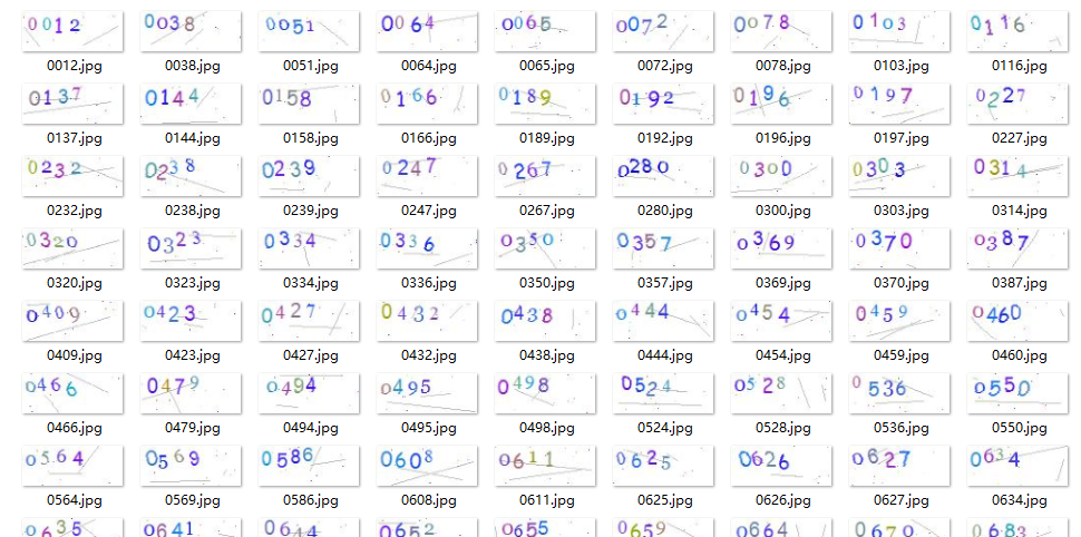
  接下来开始获取训练用的数据集，首先使用旧的 Tesseract 识别引擎，通过反复识别验证码模拟登陆，同时记录下登录成功时的识别结果，即能得到验证码和数字的对应组合：

import os
import pickle
import re
import subprocess as sp

import cv2
import httpx
import numpy as np
from loguru import logger

from binarize import split, DIGITS
from spider import get_uuid

DATASIZE = 3000
USERNAME, PASSWORD = '# 学号 #', '# 登录密码 #'
MESSAGE_LOGIN_SUCCESS = '成功'


class Spider(object):
    def __init__(self, username, password):
        self.client = httpx.Client()
        self.username = username
        self.password = password

    @staticmethod
    def ocr(image):
        proc = sp.Popen(['tesseract', '-', '-'], stdin=sp.PIPE, stdout=sp.PIPE)
        proc.stdin.write(image)
        proc.stdin.close()
        result = re.sub('[^0-9]', '', proc.stdout.read().decode())
        if len(result) != 4:
            return None
        return result

    def fetch_captcha(self):  # 获取一张验证码
        try:
            token = (
                self.client.get('https://fangkong.hnu.edu.cn/api/v1/account/getimgvcode')
            ).json()['data']['Token']
            image = self.client.get(f'https://fangkong.hnu.edu.cn/imagevcode?token={token}')
            captcha = cv2.imdecode(np.frombuffer(image.content, np.uint8), cv2.IMREAD_COLOR)
            return image.content, captcha, token
        except Exception as err:
            logger.error(repr(err))
            return None, None, None

    def verify(self, code, token):  # 验证 Tesseract 的识别结果
        try:
            result = self.client.post(
                'https://fangkong.hnu.edu.cn/api/v1/account/login',
                data={
                    'Code': self.username,
                    'Password': self.password,
                    'WechatUserInfoCode': None,
                    'VerCode': code,
                    'Token': token
                }
            ).json()
            if result['msg'] == MESSAGE_LOGIN_SUCCESS:
                return True

            logger.info(f'Login failed: {result["msg"]}')
            return False

        except Exception as err:
            logger.error(repr(err))
            return False

    def run(self, count):
        success = 0
        while success < count:
            raw_captcha, captcha, token = self.fetch_captcha()
            while captcha is None or (code := self.ocr(raw_captcha)) is None or (digits := split(captcha)) is None:
                raw_captcha, captcha, token = self.fetch_captcha()
            # noinspection PyUnboundLocalVariable
            if self.verify(code, token):
                success += 1
                for i, ch in enumerate(code):
                    with open(f'../data/marked/{ch}/{get_uuid()}', 'wb') as fp:
                        fp.write(pickle.dumps(digits[i]))
                logger.info(f'[{code}] Success.')


def main():
    spider = Spider(USERNAME, PASSWORD)
    average = sum(len(os.listdir(f'../data/marked/{n}')) for n in range(10)) / DIGITS
    logger.debug(f'Image count: {average} / {DATASIZE}')
    spider.run(max(DATASIZE - average, 0))


if __name__ == '__main__':
    main()

  挂机请求几个小时 （辅导员摇了我吧，我可是专门挑打卡低峰期来发请求的 qwq），下载到了不少验证码：

  简单检查一下结果，切分的准确程度超乎我的意料，绝大部分的字符都被准确的分类了，只有极少数出现残缺。接下来，也是整个项目最难的部分，编写神经网络……

原理分析

  我设计了一个四层的神经网络，除输入输出层外还包含两个隐含层

  输入层有 150 个神经元，两个隐含层分别有16个神经元，输出层的10个神经元分别代表 0~9 的数字，每个神经元的激活值都在 [0, 1) 区间内

  假设第 $i$ 层有 $N_i$ 个神经元第 $j$ 个神经元的激活值为 $a_i^j$，则第 $i+1$ 层第 $k$ 个神经元的激活值为:

$$a_{i+1}^k = \sum_{j=1}^{N_i}a_i^j\cdot\omega_{i+1}^{kj} + b_{i+1}^k$$

  其中 $\omega_{i+1}^{kj}$ 表示从第 $i$ 层第 $j$ 个神经元到第 $i+1$ 层第 $k$ 个神经元的激活权重（weight），$b_{i+1}^k$ 表示第 $i+1$ 层第 $k$ 个神经元的激活偏置值（bias），
这样网络的「向下传递」过程就能用矩阵运算来定义：

$$\begin{bmatrix} a_{i+1}^1 \\ a_{i+1}^2 \\ \vdots \\ a_{i+1}^m \\ \end{bmatrix} = \Omega \overrightarrow{a_i} + \overrightarrow{b_{i+1}} = Sigmoid(\begin{bmatrix} \omega_{i+1}^{11} & \omega_{i+1}^{12} & \cdots & \omega_{i+1}^{1n} \\ \omega_{i+1}^{21} & \omega_{i+1}^{22} & \cdots & \omega_{i+1}^{2n} \\ \vdots & \vdots & \ddots & \vdots \\ \omega_{i+1}^{m1} & \omega_{i+1}^{m2} & \cdots & \omega_{i+1}^{mn} \\ \end{bmatrix} \begin{bmatrix} a_i^1 \\ a_i^2 \\ \vdots \\ a_i^n \\ \end{bmatrix} + \begin{bmatrix} b_{i+1}^1 \\ b_{i+1}^2 \\ \vdots \\ b_{i+1}^m \\ \end{bmatrix})$$

  Sigmoid 为挤压函数，用于将数轴上的数压缩到 $(0, 1)$ 范围内：

$$Sigmoid(x) = \frac{1}{1+e^{-x}}$$

  定义一个代价函数，其值为每个输出激活值与期望值的差的平方和：

$$C=\sum_{i=1}^{N_{-1}}(a_{-1}^i-E_i)^2$$

  其中 $E_i$ 为输出层每个神经元的期望输出值，则我们的目标就是调整这三个矩阵中的数，使得这个代价函数取得一个局部（也有可能是全局）最小的值；这里使用一种称之为「梯度下降法」的方法，每次计算出代价函数的负梯度，然后将所有权重和偏置组成的向量沿负梯度方向调整一小步

  考虑第 i 层的第 k 个神经元，并用它的「代价」对上一层（神经元的下标用 j 表示）的权重和偏置分别求偏导数，即：

$$C_i^k = (a_i^k-E_i^k)^2 = (Sigmoid(\sum_{j=1}^{N_{i-1}}a_{i-1}^j\cdot\omega_{i}^{kj}+b_i^k)-E_i^k)^2$$

  不妨设：

$$z_i^k=\sum_{j=1}^{N_{i-1}}a_{i-1}^j\cdot\omega_{i}^{kj}+b_i^k$$

  则：

$$\frac{\partial C_i^k}{\partial \omega_{i}^{kj}} = 2(a_i^k-E_i^k) \cdot Sigmoid'(z_i^k) \cdot a_{i-1}^j$$

$$\frac{\partial C_i^k}{\partial b_i^k} = 2(a_i^k-E_i^k) \cdot Sigmoid'(z_i^k)$$

$$\frac{\partial C_i^k}{\partial a_{i-1}^j} = 2(a_i^k-E_i^k) \cdot Sigmoid'(z_i^k) \cdot \omega_{i}^{kj}$$

  这样我们就得到了输出层的一个神经元关于调整权重和偏置的「想法」以及对上一层激活值的「期望」，现在把整个过程写成矩阵运算。设 $D_i^k = 2(a_i^k-E_i^k)\cdot Sigmoid(z_i^k)$，则：

$$\nabla C(\Omega) = \begin{bmatrix} \frac{\partial C_i^1}{\partial \omega_{i}^{11}} & \frac{\partial C_i^1}{\partial \omega_{i}^{12}} & \cdots & \frac{\partial C_i^1}{\partial \omega_{i}^{1n}} \\ \frac{\partial C_i^2}{\partial \omega_{i}^{21}} & \frac{\partial C_i^2}{\partial \omega_{i}^{22}} & \cdots & \frac{\partial C_i^2}{\partial \omega_{i}^{2n}} \\ \vdots & & \ddots & \vdots \\ \frac{\partial C_i^m}{\partial \omega_{i}^{m1}} & \frac{\partial C_i^m}{\partial \omega_{i}^{m2}} & \cdots & \frac{\partial C_i^m}{\partial \omega_{i}^{mn}} \end{bmatrix} = \begin{bmatrix} D_i^1 \\ D_i^2 \\ \vdots \\ D_i^m \end{bmatrix} \begin{bmatrix} a_{i-1}^1 & a_{i-1}^2 & \cdots && a_{i-1}^n \end{bmatrix}$$

$$\nabla C(B) = \begin{bmatrix} \frac{\partial C_i^1}{\partial b_i^1} \\ \frac{\partial C_i^2}{\partial b_i^2} \\ \vdots \\ \frac{\partial C_i^m}{\partial b_i^m} \end{bmatrix} = \begin{bmatrix} D_i^1 \\ D_i^2 \\ \vdots \\ D_i^m \end{bmatrix}$$

  对整个网络的训练过程，实质上就是为所有神经元选取合适的权重和偏置，使得对于所有训练数据，代价函数的平均值尽可能小
  这里如果使用传统近似求导的办法计算代价函数对于每一个权重和偏置的偏导数，将会产生大量重复计算，极大降低了算法的效率
  但是我们学过线性代数啊，将求偏导的思想和复合函数的链式法则结合起来，以层为单位「反向传播」，就能在较优的时间复杂度内计算出梯度向量

$$\qquad \partial z_i^k = \partial b_i^k = \sum_{j=1}^{N_{i-1}}(\omega_i^{kj}\cdot Sigmoid'(z_{i-1}^j)\cdot\partial{z_{i-1}^j})$$

$$\Longrightarrow \frac{\partial z_i^k}{\partial z_{i-1}^j} = \omega_i^{kj}\cdot Sigmoid'(z_{i-1}^j)$$

  不妨设：

$$\qquad \overrightarrow{\Delta_i} = \begin{pmatrix} \frac{\partial \overline{C}}{\partial z_i^1} & \frac{\partial \overline{C}}{\partial z_i^2} & \cdots & \frac{\partial \overline{C}}{\partial z_i^{N_i}} \end{pmatrix}^T$$

$$\Longrightarrow \overrightarrow{\Delta_{i-1}}_j = Sigmoid'(z_{i-1}^j)\cdot\sum_{k=1}^{N_i}(\omega_i^{kj}\cdot\overrightarrow{\Delta_i}_k)$$

$$\Longrightarrow \overrightarrow{\Delta_{i-1}} = \begin{bmatrix} Sigmoid'(z_{i-1}^1)\cdot\sum_{k=1}^{N_i}(\omega_i^{k1}\cdot\overrightarrow{\Delta_i}_k) \\ Sigmoid'(z_{i-1}^2)\cdot\sum_{k=1}^{N_i}(\omega_i^{k2}\cdot\overrightarrow{\Delta_i}_k) \\ \vdots \\ Sigmoid'(z_{i-1}^{N_{i-1}})\cdot\sum_{k=1}^{N_i}(\omega_i^{kN_{i-1}}\cdot\overrightarrow{\Delta_i}_k) \end{bmatrix} = Sigmoid'(\begin{bmatrix} z_{i-1}^1 \\ z_{i-1}^2 \\ \vdots \\ z_{i-1}^{N_{i-1}} \end{bmatrix}) \circ (\Omega_i^T\overrightarrow{\Delta_i})$$

  这样一来就得到了各层偏导数之间的转化关系，通过 $\overrightarrow{\Delta}$ 向量，也可以轻松求出各层权重对代价函数的平均偏导（之前只求了偏置的偏导）：

$$\begin{bmatrix} \frac{\partial \overline{C}}{\partial \omega_i^{11}} & \frac{\partial \overline{C}}{\partial \omega_i^{12}} & \cdots & \frac{\partial \overline{C}}{\partial \omega_i^{2N_{i-1}}} \\ \frac{\partial \overline{C}}{\partial \omega_i^{21}} & \frac{\partial \overline{C}}{\partial \omega_i^{22}} & \cdots & \frac{\partial \overline{C}}{\partial \omega_i^{2N_{i-1}}} \\ \vdots & & \ddots & \vdots \\ \frac{\partial \overline{C}}{\partial \omega_i^{N_i1}} & \frac{\partial \overline{C}}{\partial \omega_i^{N_i2}} & \cdots & \frac{\partial \overline{C}}{\partial \omega_i^{N_iN_{i-1}}} \end{bmatrix} = \overrightarrow{\Delta_i}\begin{bmatrix} a_{i-1}^1 & a_{i-1}^2 & \cdots && a_{i-1}^n \end{bmatrix} = \overrightarrow{\Delta_i}\overrightarrow{a_{i-1}}^T$$

  至此，数学推导过程已全部完成，现在只需将数学过程转换为 Python 代码即可。

代码实现

  首先声明一个类作为神经网络的基本模型：

class NeuralNetwork:
    def __init__(self, structure=None):
        self.iterates = 0  # 记录迭代次数
        self.weights = []  # 各层权重
        self.biases = []  # 各层偏置
        self.structure = structure  # 网络结构
        self.num_layers = len(structure) if structure else 0  # 网络层数
        self.weights_buffer = []  # 权重梯度缓存
        self.biases_buffer = []  # 偏置梯度缓存
        self.loss_buffer = 0  # 损失量缓冲
        self.buffer_size = 1  # 记录缓冲大小（次数）

  接下来定义一个成员方法以初始化神经网络，当模型文件不存在时，将根据网络结构分配随机的权重与偏置值，否则从磁盘中加载模型文件作为权重与偏置；同时注册一个 onexit() 函数，程序结束时自动将本次训练的结果保存到文件中。

def init(self, filename='model.pck'):
    @atexit.register
    def onexit():
        self.structure and pickle.dump([self.weights, self.biases], open(filename, 'wb'))

    if os.path.exists(filename):
        data = pickle.load(open(filename, 'rb'))
        self.weights = data[0]
        self.biases = data[1]
    else:
        from time import time
        np.random.seed(int(time()))
        for layer in self.structure:
            self.weights.append(np.random.random(layer)*2-1)
            self.biases.append(np.random.random((layer[0], 1))*2-1)
    self.init_buffer()

  通过传入 (img, num) 组进行训练，由于 OpenCV 图片格式和我们所需要的输入数据类型不一致，首先对数据进行处理；取灰度图红色通道进行归一化、取反后化为线性，再提供给反向传播函数

def train(self, img, num):
    x, y = (1-img[:, :, 0]/255).reshape((150, 1)), np.zeros((10, 1))
    y[num] = 1
    nabla_b, nabla_w, loss = self.backprop(x, y)
    for i, b in enumerate(nabla_b):
        self.biases_buffer[i] += b
    for i, w in enumerate(nabla_w):
        self.weights_buffer[i] += w
    self.loss_buffer += loss
    self.buffer_size += 1

  重头戏来了，接下来开始实现神经网络的核心部分——反向传播函数，首先实现 Sigmoid 函数、它的导数以及代价函数的导数，接下来开始正向和反向传播过程，用 nabla_w 和 nabla_b 数组记录由本组数据计算出的梯度，最后返回两个梯度和本次计算出的代价：

@staticmethod
def sigmoid(x):
    return 1/(1+np.exp(-x))

@staticmethod
def d_sigmoid(x):
    tmp = np.exp(x)
    return tmp/(tmp+1)**2

@staticmethod
def d_loss(x, y):
    return 2*(x-y)

def backprop(self, x, y):
    # x: 输入值  y: 期望
    nabla_b = [np.zeros(b.shape) for b in self.biases]
    nabla_w = [np.zeros(w.shape) for w in self.weights]

    # 正向传递
    activation = x
    activations = [x]
    zs = []
    for b, w in zip(self.biases, self.weights):
        z = (w @ activation) + b
        zs.append(z)
        activation = self.sigmoid(z)
        activations.append(activation)
    # 反向传播
    delta = self.d_loss(activations[-1], y) * self.d_sigmoid(zs[-1])
    nabla_b[-1] = delta
    nabla_w[-1] = delta @ activations[-2].T

    for i in range(2, self.num_layers):
        sp = self.d_sigmoid(zs[-i])
        delta = (self.weights[-i+1].T @ delta) * sp
        nabla_b[-i] = delta
        nabla_w[-i] = delta @ activations[-i-1].T
    return nabla_b, nabla_w, np.sum((activations[-1]-y)**2)

  还需要一个「释放函数」用于数据集的释放和参数的更新，每个 batch 训练完成之后，调用 release() 函数即以指定训练速度向负梯度方向前进一小步：

def init_buffer(self):
    self.biases_buffer = [np.zeros(b.shape) for b in self.biases]
    self.weights_buffer = [np.zeros(w.shape) for w in self.weights]
    self.loss_buffer = 0
    self.buffer_size = 0

def release(self, rate=0.001):
    for i, b in enumerate(self.biases_buffer):
        self.biases[i] -= b * rate
    for i, w in enumerate(self.weights_buffer):
        self.weights[i] -= w * rate
    self.iterates += 1
    loss = self.loss_buffer / self.buffer_size
    print(f'[*] {self.iterates} iterations, loss: {loss}', end='\r')
    self.init_buffer()

  所有的训练都是为了识别而准备的，所以我这里实现了一个 guess() 方法，神经网络将根据当前训练的成果给出对图片中数字的猜测：

def guess(self, img):
    x = (1-img[:, :, 0]/255).reshape((150, 1))
    activation = x
    for b, w in zip(self.biases, self.weights):
        activation = self.sigmoid((w @ activation) + b)
    guess = [activation[i][0] for i in range(10)]
    return guess.index(max(guess))

  在 main() 函数中，进行模板的读取和训练：

def main():
    network = NeuralNetwork([(16, 150), (16, 16), (10, 16)])
    network.init()
    while True:
        for folder in os.listdir('models'):
            for file in os.listdir(f'models/{folder}'):
                img = cv2.imread(f'models/{folder}/{file}')
                network.train(img, int(file[0]))
            network.release()

  在实际应用过程中，非常不推荐使用 CPU 来进行训练，12 核的 CPU 在不做其他优化的情况下只能单核跑满，即使把所有核都利用上，其效率也远不如使用 GPU 训练高；不过好在识别十个数字的网络结构很简单，样本大小也不大，跑了挂着十几分钟之后已经能够基本达到使用需求

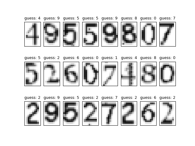
  最后随机抽取了一些字符进行测试，发现识别效果还是很不错的（至少比原来用 Tesseract 好多了），24 个字符中仅有一个 7 被识别为 1，其余结果均正确：

  将之前的内容整合一下，得到最终的验证码识别模块，简单部署一下，就可以投入使用叻：

class NeuralNetwork:
    def __init__(self):
        data = pickle.load(open('model.pck', 'rb'))
        self.weights = data[0]
        self.biases = data[1]

    @staticmethod
    def sigmoid(x):
        return 1 / (1 + np.exp(-x))

    def guess(self, img):
        x = (1-img/255).reshape((150, 1))
        activation = x
        for b, w in zip(self.biases, self.weights):
            activation = self.sigmoid((w @ activation) + b)
        result = [activation[i][0] for i in range(10)]
        return result.index(max(result))


def dfs(mask, x, y, task):
    if 0 <= x < mask.shape[0] and 0 <= y < mask.shape[1] and not mask[x][y]:
        mask[x, y] = 1
        task.put((x, y))
        for way in ((-1, 0), (0, 1), (0, -1), (1, 0)):
            dfs(mask, x+way[0], y+way[1], task)


def guess(img):
    img = cv2.cvtColor(img, cv2.COLOR_BGR2GRAY)[:27, :67]
    img = cv2.threshold(img, 180, 255, cv2.THRESH_BINARY)[1]
    mask = np.array(np.where(cv2.GaussianBlur(img, (3, 5), 0) > 210, 255, 0), dtype=np.uint8)
    count, cuts = 0, []
    for i in range(mask.shape[0]):
        for j in range(mask.shape[1]):
            area = Queue()
            minx, maxx, miny, maxy = 1 << 20, -1, 1 << 20, -1
            dfs(mask, i, j, area)
            if 20 < area.qsize() < 150:
                count += 1
                while not area.empty():
                    tmp = area.get()
                    minx = min(minx, tmp[0])
                    maxx = max(maxx, tmp[0])
                    miny = min(miny, tmp[1])
                    maxy = max(maxy, tmp[1])
                cuts.append((minx, maxx+1, miny, maxy+1))
            else:
                while not area.empty():
                    mask[area.get()] = 255
    img[np.where(mask != 1)] = 255
    cuts.sort(key=lambda s: s[2])
    network = NeuralNetwork()
    result = ''
    if count == 4:
        for i, ss in enumerate(cuts):
            digit = cv2.resize(img[ss[0]:ss[1], ss[2]:ss[3]], (2*(ss[3]-ss[2]), 2*(ss[1]-ss[0])))
            digit = cv2.resize(digit, (ss[3]-ss[2], ss[1]-ss[0]))
            template = np.full((15, 10), 255, dtype=np.uint8)
            if 3*digit.shape[1] > 2*digit.shape[0]:
                digit = cv2.resize(
                    digit,
                    (10, int(10*digit.shape[0]/digit.shape[1])),
                    interpolation=cv2.INTER_LINEAR_EXACT
                )
                dy = int((15-digit.shape[0])/2)
                template[dy:dy+digit.shape[0], :] = digit
            else:
                digit = cv2.resize(
                    digit,
                    (int(15*digit.shape[1]/digit.shape[0]), 15),
                    interpolation=cv2.INTER_LINEAR_EXACT
                )
                dx = int((10-digit.shape[1])/2)
                template[:, dx:dx+digit.shape[1]] = digit
            result += str(network.guess(template))
        return result
    else:
        return None

  最后挂一下自己的仓库地址：

GitHub

https://github.com/Mufanc/HNU-AutoCheckin

参考

• 深度学习100问之深入理解Back Propagation（反向传播）

• 深度学习之手撕神经网络代码（基于numpy）